Generative Adversarial Networks (GANs), discovered by Ian Goodfellow in 2014, were an early method in the area of generative AI. I will focus on image generation as set out in the paper Generative Adversarial Nets1. This paper is the focal point of the post, I will guide you through the implementation of the paper. After reading this I hope you understand GANs better and how to build them.
A small note, this blog post will attempt to show you my full process for understanding and implementing the paper, I hope you find this helpful. I assume some prior background knowledge of deep learning techniques, e.g. what is an MLP2, the basics of PyTorch3.
The name Generative Adversarial Network tells us a part of the story of this framework. In a GAN we have two models, the Generator (G) model and the Discriminator (D) model, which we pit against each other in a game. The goal of G is to capture the distribution of the training data and then use this to generate samples (images in our case) from that distribution. Now what does it mean for a dataset of images to have a distribution, simply the images themselves have stastical properties. In an image typically neighbouring pixels have high correlation and distant have low correlation. In MNIST specifically there is a lot of straight lines and curves (as you’d expect in images). The G model learns these statistical properties, thus learning the distribution and samples from this to generate new images.
On the other hand, the goal of D is to determine whether an image is from the training set distribution or the G distribution i.e. to detect if an image is real (a real image is one from the training set), or fake (an image from the generated set).
The training regime is as follows: the D model is trained to maximise the probability of assigning the correct label to both generated and training examples and the G model is trained to maximise the probabilty of D making a mistake (more on this later). Let’s explore the journey to arrive at the final implementation!
The Path to Implementation
A major point of confusion for me was the idea of training two neural networks simultaneously and the mechanics of this. So, first I trained just one, namely the Discriminator model. I figured that if I can get a D model which could classify between generated random noise images and real images, it would build my underlying understanding of the GAN and how to create the training loop. To get started with this lets first define the D and G models. We will only train D we will not update the parameters of G.
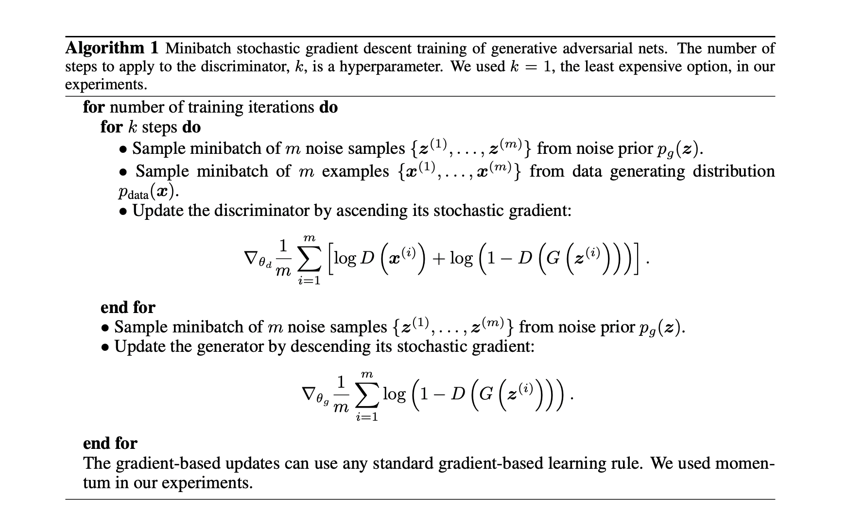
This idea came from examining Algorithm 1 provided in the paper:
Algorithm 1
We see in Algorithm 1 we have two gradient updates, initially to get our heads around the problem lets simply update the generator only.
Heads up The following is an insight into my process of understanding the paper, feel free to skip ahead to the actual implemenation.
Simple Generator
First, let’s get all the admin stuff out the way ;)
# All the imports required for this implementationimport torchimport torchvisionimport torch.nn as nnimport torchvision.transforms as transformsfrom torch.utils.data import TensorDataset, ConcatDataset, random_split, DataLoader, Datasetimport numpy as npimport matplotlib.pyplot as plt# We can make use of a GPU if you have one on your computer. This works for Nvidia and M series GPU'sif torch.backends.mps.is_available(): device = torch.device("mps")# These 2 lines assign some data on the memory of the device and output it. The output confirms# if we have set the intended device x = torch.ones(1, device=device)print (x)elif torch.backends.cuda.is_built(): device = torch.device("cuda") x = torch.ones(1, device=device)print (x)else: device = ("cpu") x = torch.ones(1, device=device)print (x)
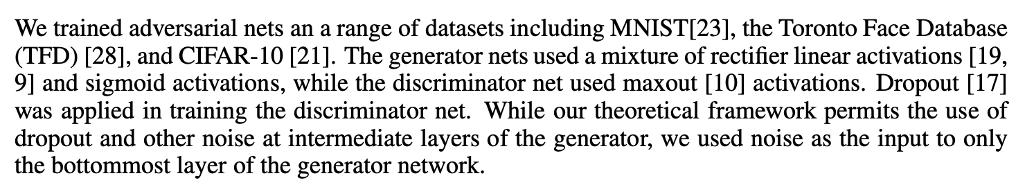
tensor([1.], device='mps:0')
I define a simple G which takes an input of size 1 and returns an image which is just random noise. In the paper it is stated that the input to G is random noise, here I choose a number from a Normal distribution as my noise and for this instance of G I set the input size to 1. Also, the ReLU layer’s in this model come from the paper, despite the actual model architecture not being specified, they state it was a a Multi-Layer Perceptron (MLP) for both D and G. For G I use a simple two layer MLP with ReLU between the layers, I also employ a tanh for the output layer. The tanh ensures the output values are between [-1, 1] this keeps our pixel values in the same range as the actual mnist data. Note, in the paper the G uses ReLU and Sigmoid but I opt for Tanh as it works better.
This is a common theme when implementing papers, you have to use your intuition when deciding the architecture and piece together the puzzle the best you can from the hints given in the paper. The papers are often incomplete in their description of the techniques used, the best way to build your intuition is doing it repeatedly and not being afraid to try different things.
To finish off, the actual output of the model must be converted to a matrix. I chose to do this inside the forward function and I include my own implementation as well as the PyTorch way. Uncomment my code to play around with it, it currently only works when the input has dimensions [1] (I leave it up to you to try and implement this to work with inputs which have more than 1 image). The reason being is that I do not handle the batch dimension, to do so you’d need another for loop.
# The following code block is a simple way to define neural networks in PyTorch.# We init the layers and then pass x through these layers in the forward pass.class Generator(nn.Module): def__init__(self):super().__init__()self.linear1 = nn.Linear(1, 256)self.relu1 = nn.ReLU()self.linear2 = nn.Linear(256, 784)self.tanh = nn.Tanh()def forward(self, x): x =self.linear1(x) x =self.relu1(x) x =self.linear2(x) x =self.tanh(x)# Need to convert the output vector x to a matrix# Note this is my way of doing the conversion, there are much better ways to do this# but, implementing it by hand may give you some insights into what is happening on line 40''' g_out_mat = torch.zeros(1, 28, 28) m = 0 n = 0 for i in range(len(x)): if i % 28 == 0 and i != 0: m += 1 n = 0 g_out_mat[0, m, n] = x[i] n += 1 '''# A simpler way to reshape the output to a 28x28 matrix# We use -1 as the first dim as it tells PyTorch to automatically calculate the correct size for x# i.e. the batch size. Try out a different value and see what happens. Functionally it is equivalent to# putting x.size(0) x = x.view(-1, 28, 28)return xgenerator = Generator()
Now lets generate a random noise sample and show what this model outputs!
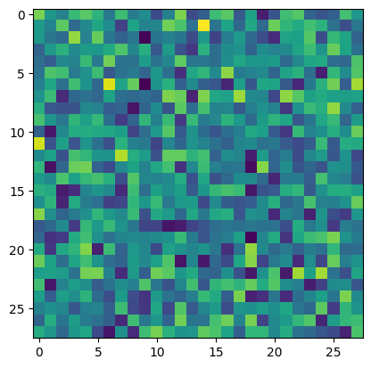
# Set mu and sigma for our Normal distrubiton and sample one value from the distributionmu, sigma =0, 1noise_value = np.random.normal(mu, sigma, 1)# The input to our network has to be a tensor datatype, in this case it just has one valueg_in = torch.tensor(noise_value, dtype=torch.float32)# We do the forward pass on the inputg_out = generator(g_in)# This is a small function to display the outputdef imshow(img): img = img /2+0.5 npimg = img.numpy() plt.imshow(np.transpose(npimg, (1, 2, 0))) plt.show()imshow(g_out.detach().cpu()), torch.Tensor([0])
We see that the image is completely random and has no patterns, which is exactly what we wanted. Now, when training the D model, we must train on both generated and real images. I was unsure on how to do this in practice, but we can use a hack in this case. Lets supplement the MNIST dataset with 60k generated images, i.e. create a 50/50 split on generated/real images.
This method is not what we use to train the actual network, as in the actual training loop we must provide newly generated samples at each epoch (the generator is improving so we want the new samples to be better at fooling the discriminator). But, for now lets stick with it!
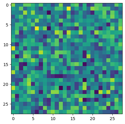
# Lets first generate 70k noise numbers from the normal distnoise_tensor = torch.randn(70000, 1)# Will pass each of these to the model to give us 70k noisy imageswith torch.no_grad(): gen_images = generator(noise_tensor) gen_images = gen_images.unsqueeze(1)gen_labels = torch.zeros((70000, 1)) # We init a list of 70k labels which are all 0. 0 means generated imagegen_labels = [0] *70000# Lets show an example of what we just generatedimshow(gen_images[0].detach()), gen_labels[0]print(f"Dimension of generated images Tensor: {gen_images.shape}")
Dimension of generated images Tensor: torch.Size([70000, 1, 28, 28])
As we wanted we get a random image just as before, only now we have 70000 of them. The next step is to add these to the original MNIST dataset. We do this as follows: create a PyTorch dataset of the generated images and their labels, create a train/test split (matching MNIST train/test split size) of the generated dataset and then finally combine the MNIST and Generated dataset together. Take a look at how this is done!
# First we need to load in the MNIST dataset. The following code is a standard way to download PyTorch# datasetsbatch_size =32# We normalise the images and convert them to tensors.transform = transforms.Compose([ transforms.ToTensor(), transforms.Normalize((0.5,), (0.5,)),])# Load both MNIST test and train setsmnist_train = torchvision.datasets.MNIST( root='./Data', train=True, download=True, transform=transform,)mnist_test = torchvision.datasets.MNIST( root='./Data', train=False, download=True, transform=transform)# For our example we are classifying if an image is from MNIST or the generated set, so we assign all examples# from MNIST with the label 1mnist_train.targets = torch.ones_like(mnist_train.targets, dtype=torch.float32)mnist_test.targets = torch.ones_like(mnist_train.targets, dtype=torch.float32)# In PyTorch we can use DataLoader class to instantiate an iterator which will efficiently pass data to the # networktrain_loader = torch.utils.data.DataLoader( mnist_train, shuffle=True, batch_size=batch_size,)test_loader = torch.utils.data.DataLoader( mnist_test, shuffle=True, batch_size=batch_size,)# TODO: We never use the train/test split why not just train with all data?
Above we load the actual MNIST dataset and now we combine the real MNIST images and the generated images.
# Create a custom dataset class which allows us to keep the labels as integers to match the MNIST data# The datatype for MNIST labels is integers, if we do not define a custom dataset class the label types# will not match up so this is necessary for the code to workclass CustomTensorDataset(Dataset):"""Dataset wrapping tensors and integer labels. Arguments: tensors (Tensor): contains sample data. labels (list of int): contains sample labels. """def__init__(self, tensors, labels):assert tensors.size(0) ==len(labels)self.tensors = tensorsself.labels = labelsdef__getitem__(self, index):returnself.tensors[index], self.labels[index]def__len__(self):returnself.tensors.size(0)gen_dataset = CustomTensorDataset(gen_images, gen_labels)# Create the train/test split of the generated datasettrain_size =60000test_size =10000gen_train_dataset, gen_test_dataset = random_split(gen_dataset, [train_size, test_size])# Combine MNIST and the generated datasetcomb_train_dataset = ConcatDataset([mnist_train, gen_train_dataset])comb_test_dataset = ConcatDataset([mnist_test, gen_test_dataset])# Create DataLoaders for the combined datasetscomb_train_loader = DataLoader(comb_train_dataset, batch_size=64, shuffle=True)comb_test_loader = DataLoader(comb_test_dataset, batch_size=64, shuffle=False)
Simple Discriminator
Now the dataset is ready to go so let’s build the classifier, AKA the Discrimanator model.
The D model is another MLP network. The input is one or more image/s and the output is a binary classification, 1 for a real image and 0 for a generated image. Again I define a somewhat arbitrary network structure, as in the case of the G model, and I once again advise you that this is a skill you will develop by trying different things when implementing these papers. In the paper it is stated that maxout activations are used, but I use ReLU and Sigmoid there isn’t a big reason why other than that it works! I understand this answer may not be satisfactory, but when implementing papers we have to test multiple avenues and find what works. I’ve found this to be the best approach for me. As I said before one of the goals is to build your intuition and it is only done through trial and error. A tip, if something doesn’t make sense like maxout activations or seems unfamiliar use something which is familiar and see if it works, sometimes you may even get better results!
To wrap up, our D model is a simple 2 layer MLP and acts as a binary classifier.
class Discriminator(nn.Module): def__init__(self):super().__init__()self.linear1 = nn.Linear(784, 256)self.relu1 = nn.ReLU()self.dropout1 = nn.Dropout(0.5)self.linear2 = nn.Linear(256, 1)self.dropout2 = nn.Dropout(0.5)# Use sigmoid to ensure output is a probability for the loss functionself.sigmoid = nn.Sigmoid()def forward(self, x): x =self.linear1(x) x =self.relu1(x) x =self.dropout1(x) x =self.linear2(x) x =self.sigmoid(x)return xdiscriminator = Discriminator()# We also send our device to the "device", i.e. the GPU if availablediscriminator.to(device)
Now we can get to the fun stuff and train our noise classifier (the D model), I call it this as we will be classifying between real images and the generated images which are noise.
First, we must choose our loss function. I use the Binary Cross Entropy Loss here, it the binary equivalent of Cross Entropy Loss. Cross Entropy Loss is a good metric for classification problems and when you implement different papers in the deep learning space you’ll come across it alot. For our purposes we just need to know it is our loss function, i.e. how good or bad our model is performing. Next we initialise our optimizer, I’ll skip over the details of this here4 (I may or may not make a post explaining all the moving parts of the training loop).
Next we setup the training loop, I have added comments to describe the role of each piece of the loop.
# An epoch just means 1 iteration, here we train for only 3 iterations. You'll see the model converges quickly# This is becuase the task is so simplefor epoch inrange(3):# Running loss keeps track of the loss at each forward/backward pass of the network, we use it to calculate# average loss of the network on each epoch running_loss =0.0# .train() sets the model to train mode, this is PyTorch behavior. You see later we have .eval() both these # methods change properties of some layers in the network. discriminator.train()# We iterate over each batch in the train_loaderfor i, data inenumerate(comb_train_loader, 0):# data is a tuple of inputs, labels so we split them up inputs, labels = data # Flatten the input, it is current a tensor of dimension (batch_size, 28, 28) # the first layer of the network expects a 784 length vector so after flattening # dimension is (batch_size, 784) inputs = torch.flatten(inputs, start_dim=1) # Push the inputs and labels to the GPU if available inputs, labels = inputs.to(device), labels.to(device)# Zero the gradients of the optimizer, this is standard in training loops# it ensures our gradient steps are not too large optimizer.zero_grad()# Perform the forward pass on our data outputs = discriminator(inputs)# Ensure outputs and labels have the same shape labels = labels.unsqueeze(1) labels = labels.float()# Calculate the loss of our network, i.e. how good/bad were it's prediction loss = criterion(outputs, labels)# Using the loss perform backpropagation loss.backward()# Using the calculated gradients bump the parameters of the model optimizer.step() running_loss += loss.item() # Print the average loss for the epochprint(f'Epoch [{epoch +1}] loss: {running_loss /len(train_loader):.3f}') running_loss =0.0# As before we set the model to eval mode discriminator.eval() correct =0 total =0# Since we're not training, we don't need to calculate the gradients for our outputswith torch.no_grad():# Perform a forward pass on the network and calculate the loss# When evaluating we do not need to calculate gradients or perform a stepfor data in comb_test_loader: images, labels = data images = torch.flatten(images, start_dim=1) labels = labels.unsqueeze(1) labels = labels.float()# Push images and labels to gpu images, labels = images.to(device), labels.to(device)# calculate outputs by running images through the network outputs = discriminator(images)# As we have 2 classes we interpret any prediction above 0.5 as a 1 and below a 0 predicted = (outputs >0.5).float() # Convert probabilities to binary predictions correct += (predicted == labels).sum().item() test_accuracy =100* correct /len(comb_test_dataset)print(f'Accuracy: {test_accuracy:.2f}%')print('Finished Training')
Observing the accuracy of the network we see 100% accuracy, this may be alarming at first but given the nature of the task it makes sense. It’s a very simple task and the network is doing well, we can verify if it works by generating a new random sample and checking the output of the network.
The output is very small, which means the model correctly classified the input as a generated image.
Success! We now have a generator which generates random images and a discriminator which can determine between generated and real images. But wait, what does this have to do with GANs? Well, the goal of a GAN is to train a D model to detect generated images and a G model to generate good generated images (or to fool the D model). What we have done above is the first step in the back and forth process, we have created a D model which can detect the poorly generated images.
The Generative Adversarial Network
Now lets extend this to implement the GAN proper!
From section 3 in the paper, the goal in training our two networks is to:
What the \(D()\) and \(D(G())\) actually refer to are the outputs of the model, however we do not mean the raw outputs but rather the output after being passed through the loss function.
So in (1) we are dealing with the D model and we are minimising the loss function of the D model. The input x consists of both real and generated images. This means we want the D model to get its classifications between generated and real images correct, we want the D model to become a better classifier.
Then in (2), we are maximising the loss of the discriminator when the inputs are generated images. The input to D is G(z), where z is random noise and G(z) being generated images. So, the loss of D(G(z)) will be high when the discriminator incorrectly classifies the generated images as real images and this is exactly what we want. Now, in practice we flip the labels of the generated images (so they have label 1 instead of 0), this allows us to turn this into a minimisation problem where we want D to classify our generated images as real. The flipping of labels and transformation to a minimisation problem also presents better gradient properties, meaning we get a better model5.
The new D and G models
Now we understand the training regime of our GAN, how do we go about implementing it? Given the nature of our task it lends us well to increase the complexity of our D and G models (they are still MLPs), I will redefine them below. My models here worked well, but feel free to add/remove layers and make your own changes and see how the output changes. Despite the changes to the models, the key differences come in the form of the new training loop.
The D model now has 4 linear layers with dropout and ReLU being applied to layers 1-3 and the output of layer 4 is passed through a Sigmoid function. This scheme arises from the paper where it is stated in section 5:
Architectural hints
Here instead of maxout activations we use ReLU within layers and Sigmoid for the output to ensure comptability with our BCE loss.
# Note the layer size choice is arbitrary in that I have no good reason for choosing it other than# that it works. This is why I advise you to play around with, e.g. see what happens if the first layer# is nn.Linear(784, 256) etc.class Discriminator(nn.Module): def__init__(self):super().__init__()self.linear1 = nn.Linear(784, 1024)self.relu1 = nn.ReLU()self.dropout1 = nn.Dropout(0.3)self.linear2 = nn.Linear(1024, 512)self.relu2 = nn.ReLU()self.dropout2 = nn.Dropout(0.3)self.linear3 = nn.Linear(512, 256)self.relu3 = nn.ReLU()self.dropout3 = nn.Dropout(0.3)self.linear4 = nn.Linear(256, 1)# Use sigmoid to ensure output is a probabilityself.sigmoid = nn.Sigmoid()def forward(self, x):# We transform the input of (batch_size, 28, 28) to (batch_size, 784) x = x.view(x.size(0), 784) x =self.linear1(x) x =self.relu1(x) x =self.dropout1(x) x =self.linear2(x) x =self.relu2(x) x =self.dropout2(x) x =self.linear3(x) x =self.relu3(x) x =self.dropout3(x) x =self.linear4(x) x =self.sigmoid(x)return xdiscriminator = Discriminator().to(device)
Similarily, the G model has 4 linear layers and it takes as input a vector of length 100. The change from input size 1 to 100 is another choice driven by empirical evidence, I’m not entirely sure why it works but my intuition is that as the task is more complex the higher dimensionality aids learning. Mess around with the size and see what happens if you make it smaller or bigger, be aware that it’s usually the case that the input size is smaller than what we are trying to generate (784 in this case).
class Generator(nn.Module): def__init__(self):super().__init__()self.linear1 = nn.Linear(100, 256)self.relu1 = nn.ReLU()self.linear2 = nn.Linear(256, 512)self.relu2 = nn.ReLU()self.linear3 = nn.Linear(512, 1024)self.relu3 = nn.ReLU()self.linear4 = nn.Linear(1024, 784)self.tanh = nn.Tanh()def forward(self, x): x =self.linear1(x) x =self.relu1(x) x =self.linear2(x) x =self.relu2(x) x =self.linear3(x) x =self.relu3(x) x =self.linear4(x) x =self.tanh(x)# Reshape the output from (batch_size, 784) to a (batch_size, 28, 28) matrix x = x.view(x.size(0), 1, 28, 28)return xgenerator = Generator().to(device)
Here we go we’re at the crux of the implementation the training loop, let’s dive right in!
# As before we use the Binary Cross Entropy Losscriterion = nn.BCELoss()# Intialise two optimisers, we use the Adam optimiser as it performs better than Stochastic Gradient Descent,# however this will work if you use Stochastic Gradient Descent as in the paper (just replace .Adam with .SGD)optimizer_D = torch.optim.Adam(discriminator.parameters(), lr=0.0001)optimizer_G = torch.optim.Adam(generator.parameters(), lr=0.0001)
Let’s look at algorithm 1 again. In algo 1 there are two loops, one lines up with ours the outer loop represents the number of epochs however we do not include the inner loop from algo 1. Our inner loop is simply iterating over our dataset and updating the model in batches. In algo 1 the inner loop has k=1 so in practice we can ignore it. The rest of algo 1 lines up with our code pretty nicely. Let’s break down each step in the algorithm and it’s representation in python:
Algorithm 1
I have numbered the key parts of Algorithm 1 and will refer to these numbers here for brevity.
1 - Corresponds to the number of training iterations or the number of epochs, so line 4 in the next code block. We run our training loop for 50 epochs, feel free to run for more/less and observe the changes in the generated images.
2 - Is the loop we ignore as k=1.
3 - Here we are simply generating our $ z $ inputs (the noise) for the G model. In line 11 of the code, we generate the tensor of noise inputs and then in line 13 we pass these to the G model to create the generated images.
4 - This step is implemented across a few lines. The algortihm does not use batches, but we do this leads to a small change in our code. Lines 5 and 6 handle the selection of the batch of data. We then need to combine these images with the generated images, the combined images will be our input to the D model. The combining of images is handled in lines 16, 17, 20, 21, 24, 25 and 26.
5 - Lines 29 - 33 handle the updating of the model. We calculate the output of the D model and update it’s parameter appropriately.
6 - We sample a new tensor of noise input in line 36 and generate the images in line 40.
7 - Lines 43 - 46 handle this, we pass the newly generated images to the updated discriminator model and then bump the gradient based on the loss of the discriminator
Thats it! We have implemented the training algorithm from the paper, all that’s left is to run the code and look at out results :)
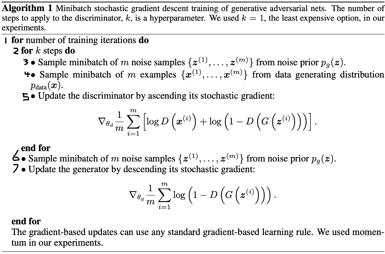
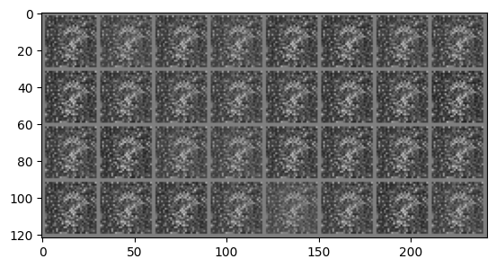
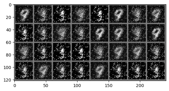
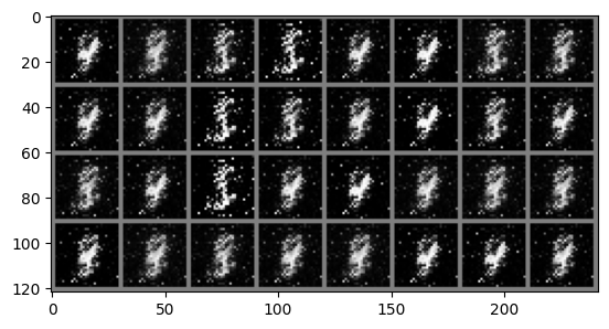
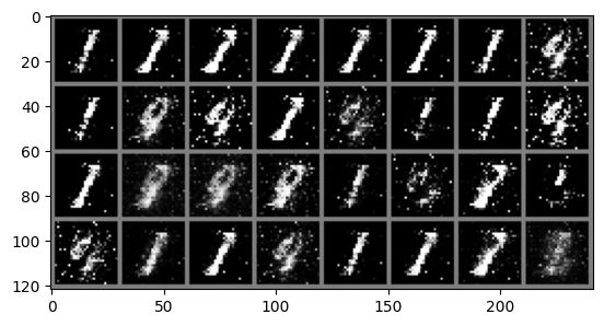
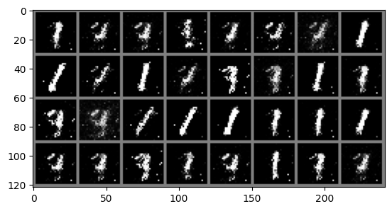
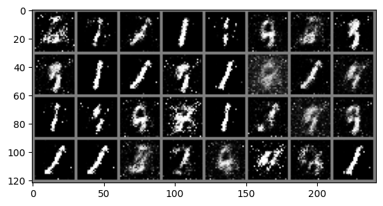
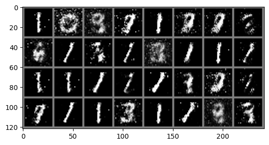
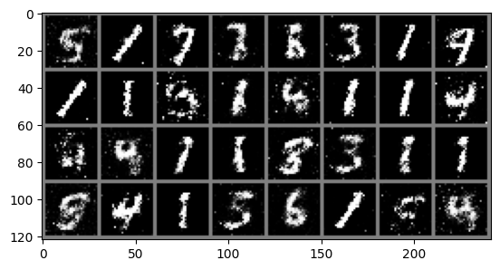
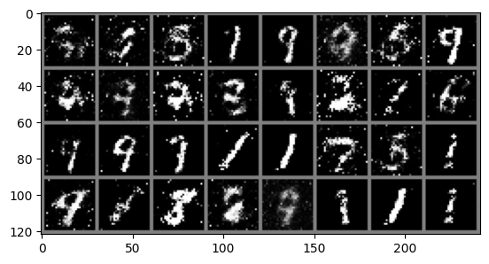
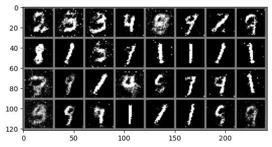
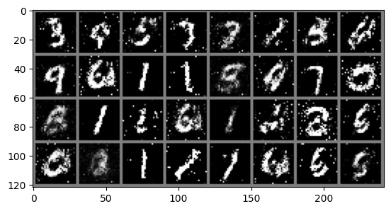
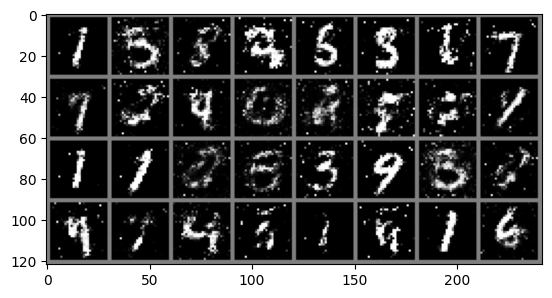
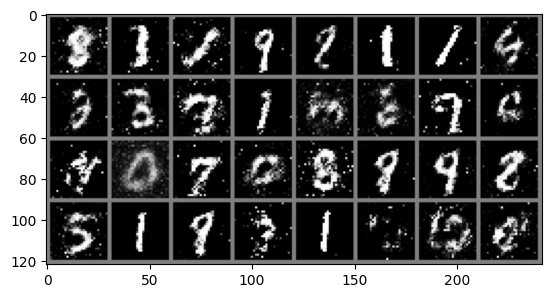
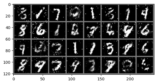
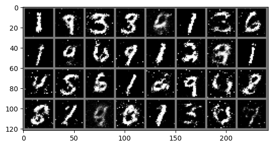
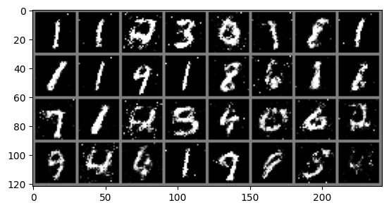
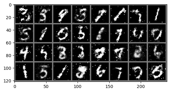
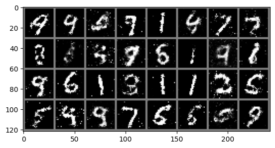
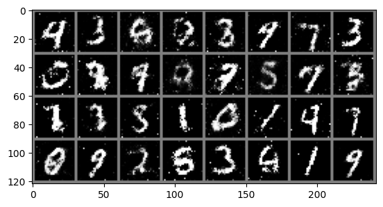
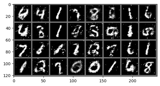
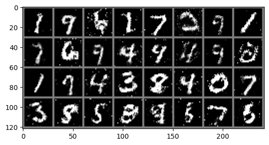
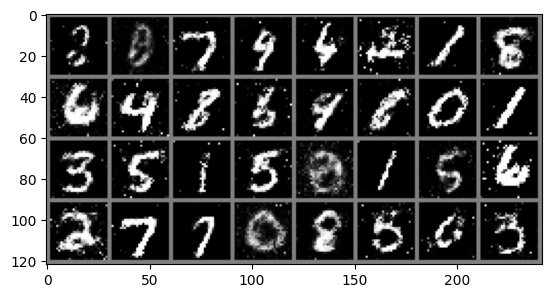
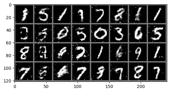
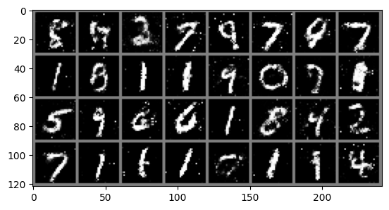
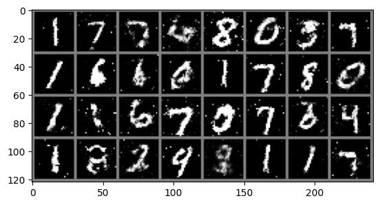
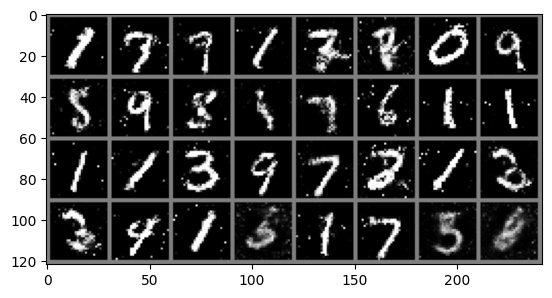
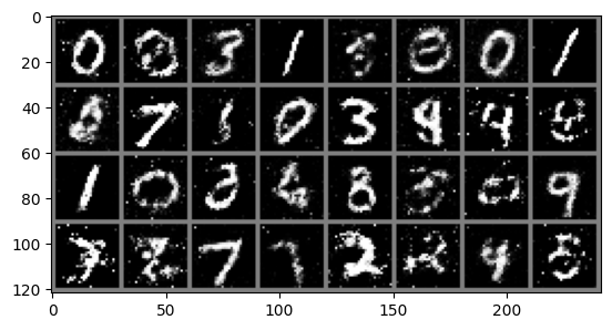
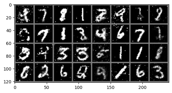
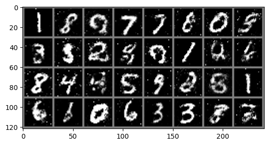
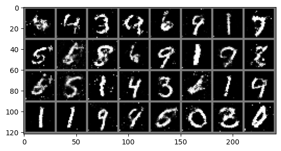
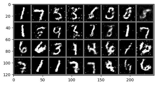
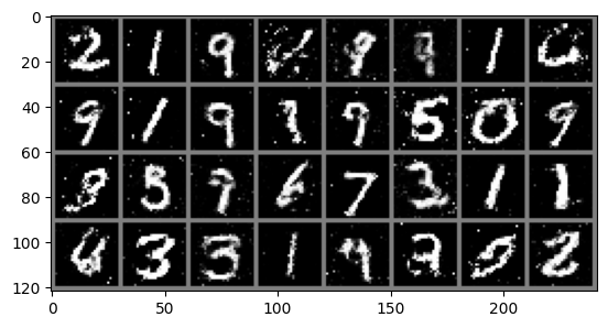
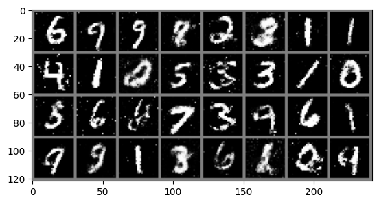
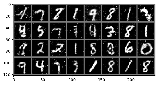
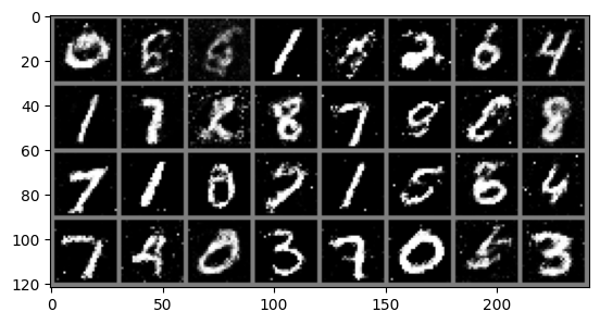
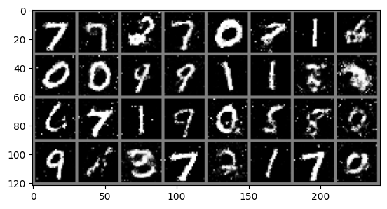
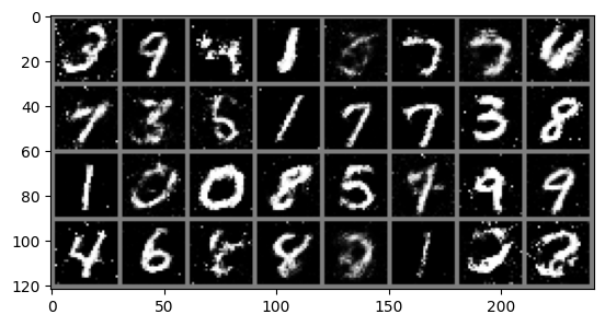
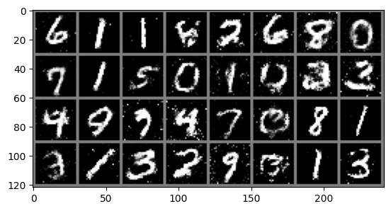
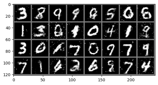
# Whenever you see a .to(device) it means we are sending that data to the GPU memory# We now run the training for 50 epochsfor epoch inrange(50):for i, data inenumerate(train_loader): real_images, _ = data # We dont care about the MNIST labels we generate a vector of all 1s to# simulate them real_images = real_images.to(device)# Sample from noise and generate the fake images noise_tensor = torch.randn((batch_size, 100)).to(device)with torch.no_grad(): gen_images = generator(noise_tensor)# Create the real and fake labels gen_labels = torch.zeros((batch_size, 1)).to(device) real_labels = torch.ones((batch_size, 1)).to(device)# Concat fake and real images combined_images = torch.cat((real_images, gen_images)) combined_labels = torch.cat((real_labels, gen_labels))# shuffle the combined batch to prevent the model from learning order indices = torch.randperm(combined_images.size(0)) combined_images = combined_images[indices] combined_labels = combined_labels[indices]# First update the D model discriminator.zero_grad() d_outputs_combined = discriminator(combined_images) loss_d = criterion(d_outputs_combined, combined_labels) loss_d.backward() optimizer_D.step()# Generate new images for updating G noise_tensor = torch.randn((batch_size, 100)).to(device)# Next update the G model, generator.zero_grad() gen_images = generator(noise_tensor) # Gen new images for training G# For generator updating we need the labels for generated images to be 1's to fool the discriminator# We do this by just passing the real_labels to the loss function# Note we use the D model, the equation in the paper is max log(D(G(z))) and we already have G(z) d_outputs_generated = discriminator(gen_images) loss_g = criterion(d_outputs_generated, real_labels) loss_g.backward() optimizer_G.step()if i == batch_size-1: '''print("g grads") for name, param in generator.named_parameters(): if param.grad is None: print(f"No gradient for {name}") elif param.grad.abs().sum() == 0: print(f"Zero gradient for {name}") else: print(param.grad) print("d grads") for name, param in discriminator.named_parameters(): if param.grad is None: print(f"No gradient for {name}") elif param.grad.abs().sum() == 0: print(f"Zero gradient for {name}") else: print(param.grad)'''print(f'Epoch {epoch}: Loss_D: {loss_d.item()}, Loss_G: {loss_g.item()}') imshow(torchvision.utils.make_grid(gen_images.cpu()))print("Training complete")
When running this code locally, there are some issues you should be aware of. Firstly, due to the stochastic nature of neural networks it is likely your generated images won’t match mine exactly. A more pressing issue can occur where the generated images all look bad and do not seem to improve, when this happens the best solution is to reinitialise the networks and run the training loop again.
Congrats, you’ve implemented and trained a GAN
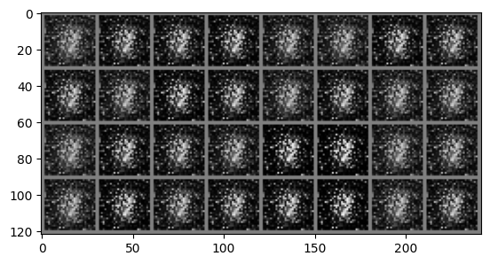
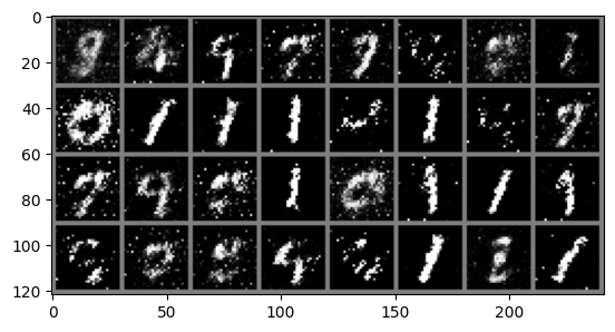
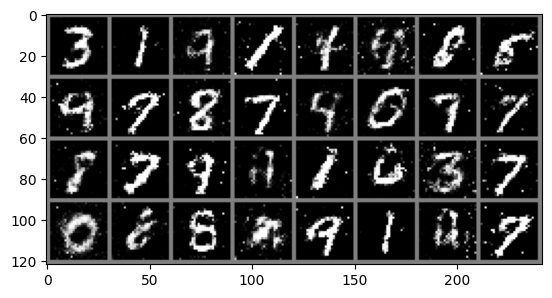
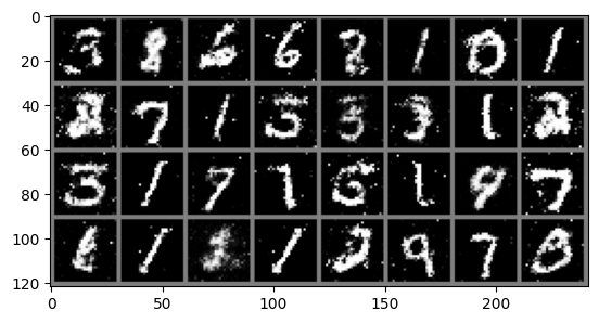
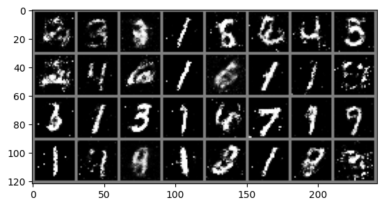
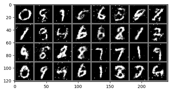
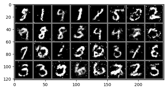
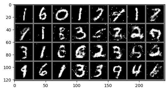
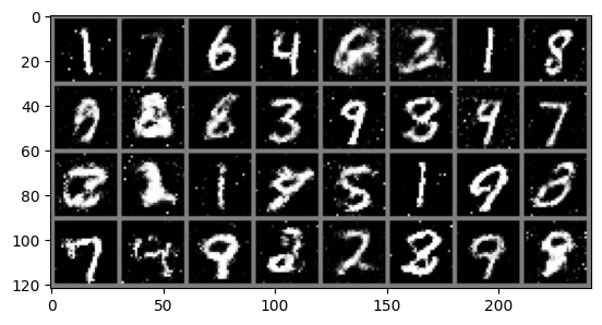
You can now see the outputs of your model and they look pretty good, perhaps you can get them to look better with more epochs or a different model architecture. Also, here’s a cool project you could try after this: traing your GAN and generate a bunch of samples of the generated digits, then build an MNIST classifier and pass these through the trained classifier and see if it gets them correct.
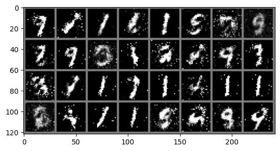
I’ll leave you with an issue with this setup of GANs. The updating of the G model is dependent upon the performance of the D model, in essence the better the feedback the D model gives the better our G model will become. However, when the G model gets good enough such that the accuracy of the D model becomes 0.5 (its guessing randomly) it’s feedback is essentially meaningless and our G model stops improving. This can be seen in our model too.
The cool idea that we should make clear is that the GAN truly does generate new images, it does not learn the training data but it generates new images. Exactly how may not be fully understood (by me anyways) but this is what is happening, isn’t that amazing!
4 I know this can be a bit frustrating to hear, but if you have any questions on this or anything discussed here feel free to reach out to me @ yusufmohammad@live.com